# Arrays.sort

这里我们主要理解一下 Java 里的 Arrays.sort 是如何实现的。

首先要知道，java中针对不同的数据类型，使用了不同的排序方法。

总体上说（不准确地说），Java 中对基本数据类型（int，short，long等）排序主要使用了 快速排序；对对象类型则使用了 归并排序。

之所以这么设计，主要有两个原因：

因为快速排序是不稳定的，而归并排序是稳定的。对于基本数据类型，稳定性没有意义，而对于对象类型，稳定性是比较重要的，因为对象相等的判断可能只是判断关键属性，所以最好保持相等对象的非关键属性的顺序与排序前一致。
归并排序相比较于快速排序，比较次数更少，移动（对象引用的移动）次数要多，而对于对象来说，比较一般比移动耗时。

上面说过这是不准确的总结。接下来，我们通过源码，具体分析一下实现。

# 基本类型的排序

这里我们以 int 类型为例，看一下具体实现。

public static void sort(int[] a) {
    DualPivotQuicksort.sort(a, 0, a.length - 1, null, 0, 0);
}

上面可以看到，主要使用了双基准快排。（其实在看源码后可以知道，其中不止有双轴快排，还使用了 TimSort，插入排序，3-way快排等）。

总体上说，该 sort 实现可以用下图表示 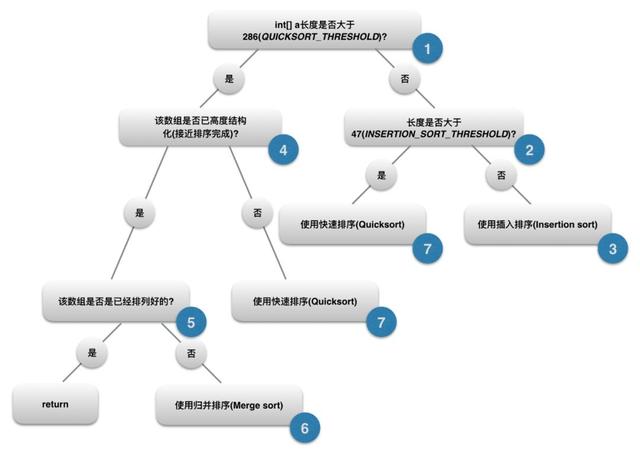dualpivotquicksort

如上图，首先判断数组的长度是否大于常量QUICKSORT_THRESHOLD，即286。当长度小于 286 时，系统将不再考虑归并排序，直接将参数传入本类中另一个私有方法sort中进行排序，执行 2.

// Use Quicksort on small arrays
if (right - left < QUICKSORT_THRESHOLD) {
    sort(a, left, right, true);
    return;
}

如上图，首先判断数组长度是否小于47.如果小于47的话，使用插入排序，否则执行到 3.

// Use insertion sort on tiny arrays
if (length < INSERTION_SORT_THRESHOLD) {
    if (leftmost) {
        /*
        * Traditional (without sentinel) insertion sort,
        * optimized for server VM, is used in case of
        * the leftmost part.
        */
        for (int i = left, j = i; i < right; j = ++i) {
            int ai = a[i + 1];
            while (ai < a[j]) {
                a[j + 1] = a[j];
                if (j-- == left) {
                    break;
                }
            }
            a[j + 1] = ai;
        }
    } else {
        /*
        * Skip the longest ascending sequence.
        */
        ......

值得注意的是，这里提供了两种不同的插入排序算法：

当传入的参数leftmost为真时，代表本次传入的数组是从最左侧left开始的，此时用的传统的没有哨兵的插入排序。
当leftmost为假时，使用了优化的插入排序，成对插入排序（具体可以看看源码）。

如上图所示，这里就是双基准排序的开始。

// Inexpensive approximation of length / 7
int seventh = (length >> 3) + (length >> 6) + 1;

首先我们看看双基准快排的大致思路，然后再从源码入手看看 JDK 中的优化和具体实现

总体思路：快速排序使用了分治的思想，将原有问题分割成若干子问题进行递归解决。在双基准快排中，顾名思义，有两个基准 pivot1, pivot2，且 pivot1 <= pivot2,然后将数组分割成三段: x < pivot1, pivot1 <= x <= pivot2, x > pivot 2。然后分别对三段进行递归，这个算法的效率通常会比传统的快排效率更高。

接下来看看具体实现。

首先是 pivot 的选取。这里，系统首先会通过位运算获取数组长度的 1/7 的近似值seventh（位运算无法精确表示 1/7）。（如上图）

然后，通过位运算获取数组的中间位置索引e3，并通过 seventh 计算中间位置的左右1/7, 2/7处，最后得到 5 个七分位点 e1, e2, e3, e4, e5.

/*
* Sort five evenly spaced elements around (and including) the
* center element in the range. These elements will be used for
* pivot selection as described below. The choice for spacing
* these elements was empirically determined to work well on
* a wide variety of inputs.
*/
int e3 = (left + right) >>> 1; // The midpoint
int e2 = e3 - seventh;
int e1 = e2 - seventh;
int e4 = e3 + seventh;
int e5 = e4 + seventh;

然后将这5个元素进行排序（插入排序）

// Sort these elements using insertion sort
if (a[e2] < a[e1]) { int t = a[e2]; a[e2] = a[e1]; a[e1] = t; }

if (a[e3] < a[e2]) { int t = a[e3]; a[e3] = a[e2]; a[e2] = t;
    if (t < a[e1]) { a[e2] = a[e1]; a[e1] = t; }
}
if (a[e4] < a[e3]) { int t = a[e4]; a[e4] = a[e3]; a[e3] = t;
    if (t < a[e2]) { a[e3] = a[e2]; a[e2] = t;
        if (t < a[e1]) { a[e2] = a[e1]; a[e1] = t; }
    }
}
if (a[e5] < a[e4]) { int t = a[e5]; a[e5] = a[e4]; a[e4] = t;
    if (t < a[e3]) { a[e4] = a[e3]; a[e3] = t;
        if (t < a[e2]) { a[e3] = a[e2]; a[e2] = t;
            if (t < a[e1]) { a[e2] = a[e1]; a[e1] = t; }
        }
    }
}

接下来，判断这5个索引对应的值是否相同：

如果5个元素的值各不相同，则选取 e2的值作为 pivot1，e4的值作为 pivot2，然后进行双基准排序。
否则，选择 e3的值作为 pivot，进行单基准排序。

if (a[e1] != a[e2] && a[e2] != a[e3] && a[e3] != a[e4] && a[e4] != a[e5]) {
    /*
    * Use the second and fourth of the five sorted elements as pivots.
    * These values are inexpensive approximations of the first and
    * second terciles of the array. Note that pivot1 <= pivot2.
    */
    ...
} else { // Partitioning with one pivot
    /*
    * Use the third of the five sorted elements as pivot.
    * This value is inexpensive approximation of the median.
    */
    ...
}

再具体的排序代码可以看源码。

接下来，我们回到 DualPivotQuicksort 开始的地方，上面都是小于 286 时的做法，下面看看大于 286 的做法。

此时，总体思路是：会判断该数组是否已经高度结构化（即是否已经接近排序完成）：如果已经接近排序完成，则使用归并排序；否则使用上面的快速排序。

那么，这里是如何判断数组是否已经高度结构化呢？具体来说，从代码可以看到：

首先会定义一个常量 MAX_RUN_COUNT = 67。
定义一个计数器 int count = 0; 定义一个数组 int[] run 使之长度为 MAX_RUN_COUNT + 1.
令 run[0] = left，然后从传入数组的左边left开始遍历，若数组的前n个元素均为升序/降序，而第 n+1 个元素的升降序发生了改变，则将第n个元素的索引存入run[1]，同时++count。
从 n+1 个元素继续遍历，直到升降序再次改变，就将此处的索引存入 run[2]，依次类推...
若将整个数组遍历完成后，count 仍然小于 MAX_RUN_COUNT（即整个数组的升降序变化低于67次），则认为数组是高度结构化的，后面会使用归并排序。而如果遍历过程中已经发现了 count == MAX_RUN_COUNT，则说明数组并非高度结构化的，会调用上面的私有方法sort进行排序。

/*
* Index run[i] is the start of i-th run
* (ascending or descending sequence).
*/
int[] run = new int[MAX_RUN_COUNT + 1];
int count = 0; run[0] = left;

// Check if the array is nearly sorted
for (int k = left; k < right; run[count] = k) {
    if (a[k] < a[k + 1]) { // ascending
        while (++k <= right && a[k - 1] <= a[k]);
    } else if (a[k] > a[k + 1]) { // descending
        while (++k <= right && a[k - 1] >= a[k]);
        for (int lo = run[count] - 1, hi = k; ++lo < --hi; ) { // 这里还会顺便将降序倒置为升序
            int t = a[lo]; a[lo] = a[hi]; a[hi] = t;
        }
    } else { // equal
        for (int m = MAX_RUN_LENGTH; ++k <= right && a[k - 1] == a[k]; ) {
            if (--m == 0) {
                sort(a, left, right, true);
                return;
            }
        }
    }

    /*
        * The array is not highly structured,
        * use Quicksort instead of merge sort.
        */
    if (++count == MAX_RUN_COUNT) {
        sort(a, left, right, true);
        return;
    }
}

后面则是归并排序的内容，具体可以看源码。

# 对象的排序

上面是以 int　类型为例介绍了 Arrays.sort() 是如何实现的。下面我们看看对于对象类型，排序是如何实现的。

首先我们要知道，对于对象类型，JDK 中主要使用了 TimSort（一种改进的归并排序）。

TimSort，其实就是结合了 MergeSort 和 InsertionSort，对 MergeSort 进行优化产生的算法，它在现实中有很好的效率，其平均时间复杂度是 O(nlogn), 最好的情况是 O(n), 最坏情况是 O(nlogn).

并且，TimSort 是一种稳定性排序，思想是先对待排序数组进行区分，然后对分区进行合并，看起来和 MergeSort 步骤一样，但是其中有一些针对反向和大规模数据的优化处理。

接下来我们看看代码

public static void sort(Object[] a) {
    if (LegacyMergeSort.userRequested)
        legacyMergeSort(a);
    else
        ComparableTimSort.sort(a, 0, a.length, null, 0, 0);
}

可以发现，先通过 LegacyMergeSort.userRequested 变量判断一下，用户是否显式要求使用遗留的归并排序：

如果要求了，那么使用遗留的归并排序。
如果用户没有显示要求，则使用优化过的 TimSort 算法。

遗留的归并排序在此不再介绍，可以直接看看源码。

下面我们看看 ComparableTimSort.sort() 是如何实现的。

static void sort(Object[] a, int lo, int hi, Object[] work, int workBase, int workLen) {
    assert a != null && lo >= 0 && lo <= hi && hi <= a.length;

    int nRemaining  = hi - lo;
    if (nRemaining < 2)
        return;  // Arrays of size 0 and 1 are always sorted

    // If array is small, do a "mini-TimSort" with no merges
    if (nRemaining < MIN_MERGE) {
        int initRunLen = countRunAndMakeAscending(a, lo, hi);
        binarySort(a, lo, hi, lo + initRunLen);
        return;
    }

首先判断待排序数组长度是不是小于2，如果小于2的话，那么数组已经是排好序的，直接返回即可；如果大于2但是小于 MIN_RANGE（其实就是32），那么执行一个叫做 mini-TimSort 的算法，它不包含合并操作，使用 binarySort。

mini-TimSort 的基本思想是：

首先从数组开始处找到一组升序或严格降序的数（如果为降序，找到后直接翻转为升序）。（即 countRunAndMakeAscending）
然后执行 binarySort(a, lo, hi, lo + initRunLen). binarySort的基本思想是：因为[lo, lo+initRunlen]这一区间已经排好序了，所以将[lo+initRunlen, hi]这一部分的元素逐一采用“二分”的方式插入进[lo, lo+initRunlen] 即可。 (具体可以看 binarySort 的代码)

然后我们回来看看，当待排序数组大于阈值 MIN_MERGE 时，就是 JDK 中使用 TimSort 的时候了。

TimSort 的基本思想是：将数据按照升序和降序的特点进行分区（如果是降序的话，直接翻转成升序），每一个分区称为一个 run，然后按归并的原则合并这些 run。

其主要代码是下面这一块：

/**
* March over the array once, left to right, finding natural runs,
* extending short natural runs to minRun elements, and merging runs
* to maintain stack invariant.
*/
ComparableTimSort ts = new ComparableTimSort(a, work, workBase, workLen);
int minRun = minRunLength(nRemaining);
do {
    // Identify next run  这里就是用来寻找 升序或降序的 分区（run）
    int runLen = countRunAndMakeAscending(a, lo, hi);

    // If run is short, extend to min(minRun, nRemaining)
    if (runLen < minRun) {
        int force = nRemaining <= minRun ? nRemaining : minRun;
        binarySort(a, lo, lo + force, lo + runLen);
        runLen = force;
    }

    // Push run onto pending-run stack, and maybe merge 这里将分区入栈
    ts.pushRun(lo, runLen);
    ts.mergeCollapse();

    // Advance to find next run  接着寻找下一个分区
    lo += runLen;
    nRemaining -= runLen;
} while (nRemaining != 0);

// Merge all remaining runs to complete sort
assert lo == hi;
ts.mergeForceCollapse();  // 最后合并所有分区，至只有一个分区，那么就已经排好序了。

总结：TimSort 是一种混合的稳定排序算法，相当于是归并排序和插入排序的改进版，对归并排序在已经反向排好序的输入时做了特别优化，对已经正向排好序的输入也可以减少回溯，对两种情况的混合（一会升序一会降序）的输入处理比较好。

← HashMap String →